Microsoft Excel
Excel is renowned for its popularity and efficiency, stands as the go-to spreadsheet software for managing substantial data. The marvel lies in its ability to seamlessly store, analyze, and report vast amounts of information. It’s a testament to human ingenuity that such comprehensive tools exist, enabling us to navigate the complexities of data management with ease. There 365 built in functions are in Excel. Among those we have covered only Xlookup in Excel, Complete guide on how to use it.
XLOOKUP in Excel
XLOOKUP is a versatile and powerful function in Microsoft Excel, introduced in Excel 365 (2019). The XLOOKUP function searches a range or an array, and then returns the item corresponding to the first match it finds. If no match exists, then XLOOKUP can return the closest match.
Here’s a basic syntax of the XLOOKUP function:
Syntax:
=XLOOKUP(lookup_value, lookup_array, return_array, [if_not_found], [match_mode], [search_mode])
Here’s what each argument means:
lookup_value: The value you want to search for.
lookup_array: The range or array where you’re searching.
return_array: The range or array from which you want to retrieve a result.
[if_not_found]: Optional. Specify a custom message when no valid match is found.
[match_mode]: Optional. Choose the type of match (exact, next smaller, next larger, or wildcard).
[search_mode]: Optional. Specify the search order (top to bottom, bottom to top, or binary search).
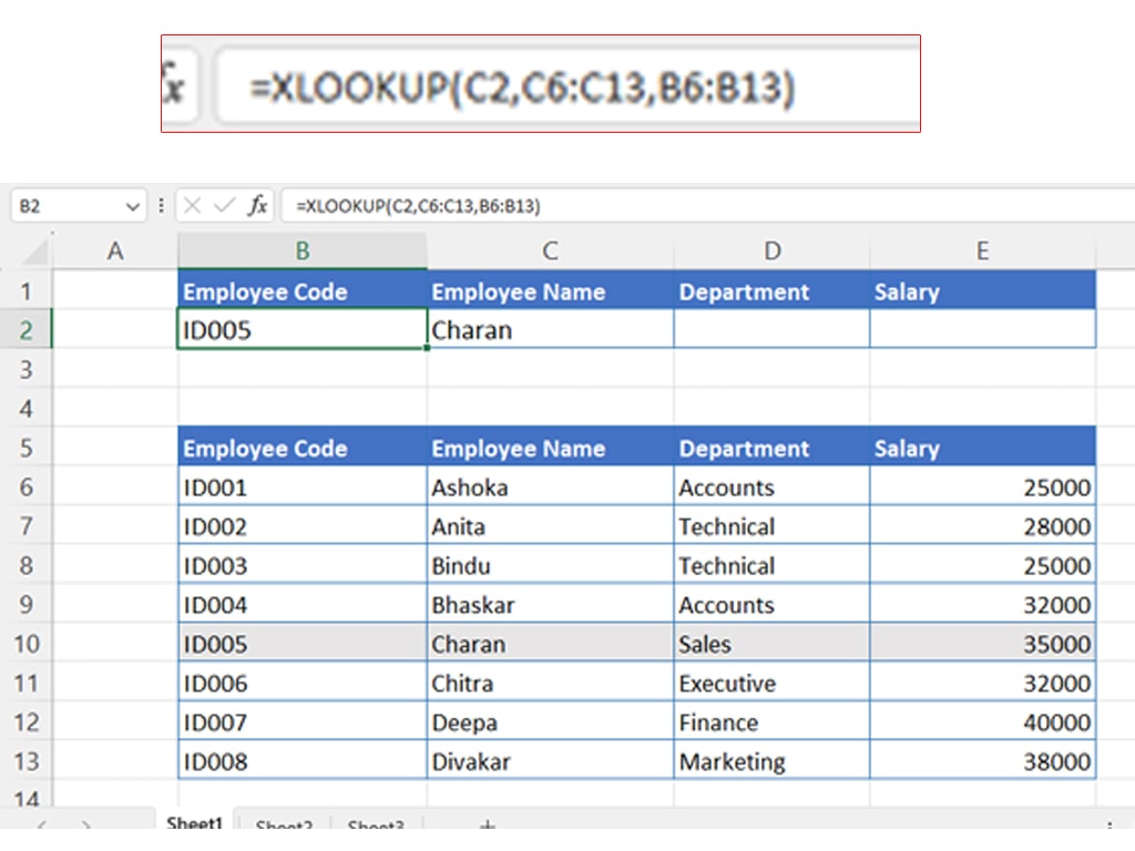
Example 1 uses XLOOKUP to look up a Employee name in a range, and then return his/her Empcode.

In this example we are searching for EmpCode in cell B2 the formula is as follows
=XLOOKUP(C2,C6:C13,B6:B13)
where,
C2 (Charan) is the value being searched for within the range or array C6:C13 (Employee Names Column), and B6:B13 is the range that returns the array where the value is found.
Note: XLOOKUP uses a lookup array and a return array, whereas VLOOKUP uses a single table array followed by a column index number. The equivalent VLOOKUP formula in this case would be: =VLOOKUP(F2,B2:D11,3,FALSE)
Example 2 looks up employee information based on an employee ID number. Unlike VLOOKUP, XLOOKUP can return an array with multiple items, so a single formula can return both employee name , department and Salary from cells C6:E13
Example 3 adds an if_not_found argument to the preceding example.
In this example the value to be found is Employee Code ID0025, which is not exists in the list.
Example 4 The match_mode argument is set to 1, which means the function will look for an exact match, and if it can’t find one, it returns the next larger item. Finally, the search_mode argument is set to 1, which means the function will search from the first item to the last.
Example 5: XLookUp replaces Hlookup function
In this example the search has been made horizontally.
Example 6: Nesting of xlookup
XLOOKUP(C2, B6:B8, XLOOKUP(B3, C5:F5, C6:F8)): This is a nested XLOOKUP formula.
- XLOOKUP(B3, C5:F5, C6:F8): This part of the formula looks for the value in cell B3 within the range C5:F5. If a match is found, it returns the corresponding value from the same column where the match is found in the range C6:F8.
- XLOOKUP(C2, B6:B8, …): The outer XLOOKUP then searches for the value in cell C2 within the range B6:B8. If a match is found, it returns the corresponding value from the same position where the match is found in the result array of the nested XLOOKUP.
- Learn How to remove duplicates in EXCEL
- How to freeze a row in Excel
- How to Use Flash Fill in Excel
- How to Use XLOOKUP in Excel
- If you wish to know more about built in Functions click this.
As you continue to explore and utilize XLOOKUP in your projects, feel free to experiment with different scenarios and leverage its features creatively. Its flexibility and versatility empower you to tackle diverse data lookup challenges with confidence and ease.
In summary, XLOOKUP represents a transformative addition to Excel’s functionality, providing a modern, intuitive, and efficient solution for all your lookup requirements. Embrace its capabilities and unleash the full potential of your Excel spreadsheets.